Configuration Space II

Keywords: Configuration Space, Topology, Holonomic Constarint, Nonholonomic Constarint, Pfaffian Constarint

I. Configuration Space Topology

앞선 챕터까지는 configuration space(이하 C-space)의 dimension(i.e. DoF)에 집중해왔다. 이 챕터에서는 C-space의 “형상”에 대한 내용을 다룬다. C-space의 형상이라니 이게 뭔 뚱딴지 같은 소리인가 싶은데, 예제를 통해 살펴보면 직관적으로 이해할 수 있다.

가령, 아래와 같이 2개의 C-space가 있다고 가정해보자.

\(\mathbf{E}^{1}\): 평면 위를 움직이는 한 점
\(\mathbf{S}^{2}\): 구의 표면 위를 움직이는 한 점

전자는 \((x, y)\)와 같이 Euclidean 좌표로, 후자의 경우 \((latitude, longitude)\)와 같이 C-space의 각 configuration을 표현해줄 수 있다. 따라서, \(\mathbf{E}^{1}\), \(\mathbf{S}^{2}\) 모두 C-space의 dimension은 2로 동일하다.

그런데, 직관적으로만 생각해보아도 C-space의 형상은 두 개가 다르지 않은가? \(\mathbf{E}^{1}\)은 무한히 뻗어나가는 평면이고, \(\mathbf{S}^{2}\)는 구의 중심을 감싸는 형태로 무한히 뻗어나가지는 못한다. 이렇듯, C-space의 형상은 DoF가 같다고 하다라도 다를 수 있다.

엄밀하게 C-space의 형상은 topology라는 개념을 통해 표현된다. 다만, 이 책은 위상수학 교과서가 아니기 때문에 아주 엄밀한 정의는 도입하지 않았고 아래와 같이 “동일한 topology를“가 무엇인지를 정의하였다.

Topologically equivalent

C-space A의 형상이 cutting이나 gluing 없이 C-space B로 변형될 수 있다면 A와 B는 topologically equivalent하다.

위의 정의는 (어릴적 해보았을) 지점토 놀이를 떠올리면 받아들이기 수월한데, 아래 움짤이 이를 표현하고 있다. 아래 그림에서 커피잔은 cutting이나 gluing 없이 도넛으로 변형되었고, 따라서 도넛과 커피잔은 topologically equivalent하다.

II. Configuration Space Representation

이제 C-space를 어떻게 “표현”할지에 대해서 고민해보자. 바로 위 챕터에서 예시하였던 \(\mathbf{S}^{2}\)를 떠올려보고 이를 표현하는 방법에 대해서 생각해보자.

\(\mathbf{S}^{2}\)는 \((latitude, longitude)\)로 각 configuration을 표현해줄 수 있다. \(\mathbf{S}^{2}\)의 DoF는 2이므로, configuration을 표현하는데 사용한 실수의 갯수와 DoF가 같다. 이렇게 표현하고자 하는 C-space의 DoF와 동일한 갯수의 실수로 configuration을 표현하는 것을 explicit parametrization이라고 부른다.
한편, \(\mathbf{S}^{2}\)는 해당 위치의 좌표를 \((x, y, z)\)로 표현해줄 수도 있다. 이 경우는 explicit parametrization과 달리 DoF보다 많은 갯수의 실수들로 각 configuration을 표현하게 된다. 이와 같이 C-space의 DoF보다 많은 갯수의 실수로 configuration을 표현하는 것을 implicit parametrization이라고 부른다.

여기까지 읽으면, “아니 대체 뭐하러 implicit parametrization을 사용하나?”와 같은 의문이 든다. 책에서는 implicit parametrization을 사용하는 것이 singularity를 다루기에 보다 편하기 때문이라고 설명하고 있다.

예를 들어, 아래 그림이 표현하는 \(\mathbf{S}^{2}\)에서 하나의 configuration이 북극(?) 근방에서 움찔움찔 움직이고 있다고 가정해보자. 아주 살짝의 움직임이더라도, 북극을 통과하게 된다면 longitude-latitude 평면에서는 포인트가 점프하는 것과 같이 표현될 것이다. 이러한 특이점을 singularity라고 부르는데, 풀고자하는 문제의 C-space에 singluarity가 존재하면 매번 특수하게 처리를 해주어야한다. 반면, 조금 비효율적이더라도 implicit parametrization을 사용하면 singularity가 해소되어 보다 편하게 문제를 풀 수 있다.

III. Holonomic vs. Nonholonomic Constraints

책의 구성을 엄밀하게 따른다면, 이 절의 title은 III. Configuration and Velocity Constraints가 되어야한다. 그런데, 아직은 (배움이 부족해서 그런 것인지) 이 절의 title이 왜 그렇게 지어진 것인지 아직은 와닿지 않는다. 그래서, 이 절의 title을 Holonomic vs. Nonholonomic Constraints로 변경하였고 기술의 순서를 조금 변경하였다.

Holonomic constraints

Reachable한 C-space를 제한해버려서, 결국 C-space의 dimension을 감소시키는 제약들을 holonomic constraint라고 부른다. 조금 더 직관적으로 설명하자면 holonomic constraints으로 인해서 로봇이 가질 수 없는 configuration이 생겨난다. 뒤에 이어질 four-bar linkage의 예제에서 보다 자세히 살펴볼 것 이다.

Nonholonomic constraints

엄밀하게 설명하면 “holonomic constraint가 아닌 것” 정도로 성의 없게 밖에 설명하지 못한다. 조금 성의 있게 설명하면, C-space의 dimension을 감소시키지는 않지만, velocity space의 dimension을 감소시키는 제약들이다. 다만, 책에서는 velocity space가 뭔지 정확히 표현되어 있지 않다. 하지만, 문맥상 configuration의 time derivative로 해석하면 이후 내용을 이해하는데 무리가 없다. 뒤에 이어지는 rolling coin의 예제에서 보다 자세히 살펴볼 것이다.

III.1. Holonomic Constraints on Planar Four-bar Linkage

책에서는 holonomic constraint의 설명을 위해서 아래의 planar four-bar linkage를 예시하고 있다.

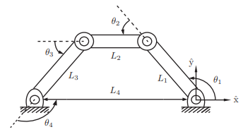
위의 예제에 적용되는 constraint들은 아래와 같이 3개의 독립적인 equation으로 표현해줄 수 있다.

\[\begin{align*} L_{1} cos(\theta_{1}) + L_{2} cos(\theta_{1} + \theta_{2}) + ... + L_{4} cos(\theta_{1} + \theta_{2} + ... + \theta_{4}) & = 0 \\ L_{1} sin(\theta_{1}) + L_{2} sin(\theta_{1} + \theta_{2}) + ... + L_{4} sin(\theta_{1} + \theta_{2} + ... + \theta_{4}) & = 0 \\ \theta_{1} + \theta_{2} + ... + \theta_{4} - 2 \pi & = 0 \end{align*}\]

고백하면, 나는 위의 우아한 constraint들을 four-bar linkage를 보고 떠올려내지 못했다. 하지만, 굳이 스트레스 받아가며 contraint의 도출 과정을 들여다보지는 않았다. 다만, 중요하다고 생각하는 점은 “왜 3개의 contraint가 도출되었는가?” 정도였고, 그 이유는 다음과 같다.

four-bar linkage 예제는 configurtaion을 4개의 실수(\(\theta_{1}, ... , \theta_{4}\))로 표현했다.

four-bar linkage 예제를 앞선 챕터에서 배운 Grubler’s Formula에 넣어주면 \(DoF = 3 \cdot (4 - 1 - 4) + 1 \cdot 4 = 1\)임을 알 수 있다.

따라서, 4개의 실수를 사용한 implicit parametrization을 1 DoF로 줄여주기 위해서는 3개의 independent contraint가 찾아져야 한다.

한편, 위의 constraint는 조금 더 general하게 아래와 같은 형태로 표현해 줄 수 있다.

\[g(\theta_{1}, \theta_{2}, \cdots, \theta_{n}) = \left[ { \begin{array}{c} g_{1}(\theta_{1}, \theta_{2}, \cdots, \theta_{n}) \\ g_{2}(\theta_{1}, \theta_{2}, \cdots, \theta_{n}) \\ \vdots \\ g_{k}(\theta_{1}, \theta_{2}, \cdots, \theta_{n}) \\ \end{array} } \right] = \mathbf{0}\]

위의 식에 등장하는 \(k\)개의 constraint는 note에서 이야기 한 것 같이, C-space의 dimension을 \(n\)에서 \(n-k\)로 감소시켜준다. 이것이 바로 holonomic constraint의 예이다.

holonimic constriant에 대한 설명은 딱 위의 문단까지해서 마무리할 수 있다. 하지만, 바로 이어서 기술할 nonholonomic constraint를 위해서 조금만 더 calculus를 해보자.

\(\Theta = (\theta_{1}, \theta_{2}, \cdots, \theta_{n})\)라고하고, 위에서 언급한 constraint의 양변을 시간(\(t\))에 대해서 미분해보면 아래를 얻을 수 있다.

\[\frac{d}{dt} g(\Theta) = \left[ { \begin{array}{c} \frac{\partial g_{1}(\Theta)}{\partial \theta_{1}} \dot{\theta_{1}} + \frac{\partial g_{1}(\Theta)}{\partial \theta_{2}} \dot{\theta_{2}} + \cdots + \frac{\partial g_{1}(\Theta)}{\partial \theta_{n}} \dot{\theta_{n}} \\ \frac{\partial g_{2}(\Theta)}{\partial \theta_{1}} \dot{\theta_{1}} + \frac{\partial g_{2}(\Theta)}{\partial \theta_{2}} \dot{\theta_{2}} + \cdots + \frac{\partial g_{2}(\Theta)}{\partial \theta_{n}} \dot{\theta_{n}} \\ \vdots \\ \frac{\partial g_{k}(\Theta)}{\partial \theta_{1}} \dot{\theta_{1}} + \frac{\partial g_{k}(\Theta)}{\partial \theta_{2}} \dot{\theta_{2}} + \cdots + \frac{\partial g_{k}(\Theta)}{\partial \theta_{n}} \dot{\theta_{n}} \\ \end{array} } \right] = \mathbf{0}\]

이것을 다시 matrix form으로 조금 변경시켜주면 아래를 얻을 수 있다.

\[\left[ { \begin{array}{cccc} \frac{\partial g_{1}(\Theta)}{\partial \theta_{1}} & \frac{\partial g_{1}(\Theta)}{\partial \theta_{2}} & \cdots & \frac{\partial g_{1}(\Theta)}{\partial \theta_{n}} \\ \frac{\partial g_{2}(\Theta)}{\partial \theta_{1}} & \frac{\partial g_{2}(\Theta)}{\partial \theta_{2}} & \cdots & \frac{\partial g_{2}(\Theta)}{\partial \theta_{n}} \\ \vdots & \vdots & \vdots & \vdots \\ \frac{\partial g_{k}(\Theta)}{\partial \theta_{1}} & \frac{\partial g_{k}(\Theta)}{\partial \theta_{2}} & \cdots & \frac{\partial g_{k}(\Theta)}{\partial \theta_{n}} \\ \end{array} } \right] \left[ { \begin{array}{c} \dot{\theta_{1}} \\ \dot{\theta_{2}} \\ \vdots \\ \dot{\theta_{n}} \\ \end{array} } \right] = \mathbf{0}\]

위 식의 좌변을 잘 살펴보면 \(\mathbf{A}(\Theta) \cdot \dot{\Theta}\)의 형태가 되는 것을 알 수 있다. 여기서 configurtaion의 time derivative(i.e. \(\dot{\Theta}\))에 곱해지는 행렬 \(\mathbf{A}(\Theta)\)를 Pfaffian constraint matrix라고 부른다. 자명하게, (적분이 가능한 경우에는) \(\mathbf{A}(\Theta)\)를 적분하면 원식이었던 holonomic constraint를 얻을 수 있으므로 holonomic constraint는 integrable constraint라고도 불린다. 적분이 불가능한 경우도 당연히 존재하고, 그러한 nonintegrable constraint는 nonholonomic constraint가 된다. 이러한 경우는 다음 절의 rolling coin 예제에서 살펴보도록하자.

III.1. Nonholonomic Constraints on Rolling Coin

책에서는 아래의 rolling coin 예제를 통해 nonholonomic constraint를 설명한다.

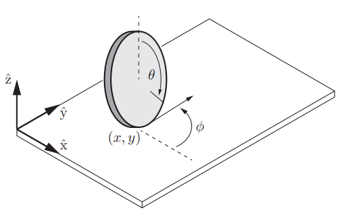
위 예제에서 동전이 평면 위에서 미끄러지 않는다고 가정을 하면 동전이 속력은 동전의 반지름을 \(r\)이라고 할 때, \(r\dot{\theta}\)가 된다. 따라서, lateral/longitudinal velocity에 대한 아래의 관계를 얻을 수 있다.

\[\begin{align*} \left[ { \begin{array}{c} \dot{x} \\ \dot{y} \\ \end{array} } \right] = r \dot{\theta} \left[ { \begin{array}{c} cos(\phi) \\ sin(\phi) \\ \end{array} } \right] \end{align*}\]

그리고, 위에서 얻어진 관계를 조금만 더 공들여 정리하면 Pfaffian constraint matrix \(A([x, y, \phi, \theta]^T)\)를 아래와 같이 구할 수 있다.

\[\begin{align*} \left[ { \begin{array}{cccc} 1 & 0 & 0 & -r cos(\phi) \\ 0 & 1 & 0 & -r sin(\phi) \\ \end{array} } \right] \left[ { \begin{array}{c} \dot{x} \\ \dot{y} \\ \dot{\phi} \\ \dot{\theta} \\ \end{array} } \right] = A([x, y, \phi, \theta]^T) \left[ { \begin{array}{c} \dot{x} \\ \dot{y} \\ \dot{\phi} \\ \dot{\theta} \\ \end{array} } \right] = \mathbf{0} \end{align*}\]

여기서 얻어진 Pfaffian constraint matrix \(A([x, y, \phi, \theta]^T)\)는 III.1의 four-bar linkage의 Pfaffian constraint matrix와 달리 적분이 불가능하다.

“아니 왜 적분이 불가능하다는 거지?” 싶다면 아래를 차근 차근 잘 살펴보도록하자. 일단, Pfaffian constraint matrix의 정의로부터 아래를 알 수 있다.

\[\begin{align*} \left[ { \begin{array}{cccc} 1 & 0 & 0 & -r cos(\phi) \\ 0 & 1 & 0 & -r sin(\phi) \\ \end{array} } \right] = \left[ { \begin{array}{cccc} \frac{\partial g_{1}}{\partial x} & \frac{\partial g_{1}}{\partial y} & \frac{\partial g_{1}}{\partial \phi} & \frac{\partial g_{1}}{\partial \theta} \\ \frac{\partial g_{2}}{\partial x} & \frac{\partial g_{2}}{\partial y} & \frac{\partial g_{2}}{\partial \phi} & \frac{\partial g_{2}}{\partial \theta} \\ \end{array} } \right] \end{align*}\]

\(g_{1}\)에만 초점을 맞추어 살펴보자. \(\frac{\partial g_{1}}{\partial \phi} = 0\)로부터, \(g_{1}\)은 \(\phi\)항을 갖지 않는 함수, 즉, \(h(x, y, \theta)\)의 형태여야 함을 알 수 있다. 그런데, \(\frac{\partial g_{1}}{\partial \theta} = -r cos(\phi)\)로부터 \(g_{1}\)은 반드시 \(-r sin(\phi) \theta\)로 정의되는 \(\phi\) 항을 가져야만 한다. 따라서, 이를 만족하는 \(g_{1}\)은 존재할 수 없고, 적분이 불가능하다.

이와 같이 적분이 불가능한 Pffafian constraint를 nonholonomic constriant라고 부른다.

III.3. Mini-summary

로보틱스를 전공하지 않은 사람으로서 평소에 holonomic constraint(혹은 nonholonomic constraint)가 대체 무엇인지 늘 궁금했었던 것 같다. 또, 구글링해서 나오는 정의들은 너무 현학적인 나머지 직관적으로 전혀 와닿지 않았었다. 지금도 이를 완벽하게 이해했다는 생각은 들지 않지만, 적어도 이제는 조금은 더 직관적인 설명을 할 수 있을 것 같다.

holonomic constraint는 이 제약으로 인해서 reachable하지 못한 configuration이 생겨난다.

예를 들어, four-bar linkage의 예제에서 \(\theta_{1} = \pi, \theta_{2} = -\frac{\pi}{2}\)인 configuration은 reachable하지 않다.

따라서, holonomic constraint는 configuration space의 dimension을 감소시킨다.

nonholonomic constraint는 holonomic constraint가 아닌 모든 제약들이고, reachable하지 못한 configuration을 만들어내지는 않는다.

다만, configuration A에서 configuration B로 이동할 때 그러한 이동이 가능한지 아닌지를 제약한다.

이 제약들로 인해 A가 B로 이동할 때 A -> X -> Y -> … -> B와 같이 복잡한 과정을 거쳐야 할 수 있다.

하지만, 엄연히 B 역시도 reachable한 configuration이다.